Risk Analysis I
Updated 2018-07-22
Risk Analysis I
Values are described in possible ranges as estimations are inheriantly uncertain. Using sentivity analysis can yield how changes in variables affect the economic analysis.
Probability is used to consider varing data, and is based on theory, historical data, judgement, or a combination. Variables with a probability are uncertain (random / stochastic) as opposed to certain (deterministic).
Review the notes on probability, conditional probability, and random variables. (ELEC 321 Notes - Stochastic Signals and Systems - UBC 2017)
- In engineeing ecnomics, it is usual to have only 2-5 discrete outcomes. This is because additional outcomes require more analysis and expert judgement should limits the number of outcomes.
- The probability of an outcome is determined by its steady-state (long-run) frequency of its occurence.
Joint Probability Distribution
Random variables are statistically independent - that is, the result of an outcome for one random variable, won’t affect the realization of another random variable. A project criteria (NPV or IRR) depends on various input variables. Thus we have to consider the joint probability distribution of different combinations of input parameters.
Recall the joint probability of two independent events is given as:
\[\mathbb P(A\cap B)=\mathbb P (A)\cdot \mathbb P(B)\]Example: oil company
Suppose the oil company has the following outcome:
Outcome Probability Well being dry :cry: 70% Well being productive :smile: 25% Well being highly producitve :joy::ok_hand::100: 5% But also the oil company has the following outcome for oil prices:
Outcome Probability Rise in oil price :thumbsup: 60% Fall in oil price :thumbsdown: 40% Then there are \(2\times 3=6\) total combinations of outcomes. The probability for each one is as follows:
Joint outcome Joint probability :cry: and :thumbsup: \(70\%\times 40\%=28\%\) :cry: and :thumbsdown: 42% :smile: and :thumbsup: 10% :smile: and :thumbsdown: 15% :joy::ok_hand::100: and :thumbsup: 2% :joy::ok_hand::100: and :thumbsdown: 3%
Expected Value
Recall from random variables notes that the general equation for expected value is the sum of weighted average based on the probability of occurance:
\[\mathbb E[g(X)]=\sum_{x}g(x)f(x)\]where \(X\) is the random variable, \(g(x)\) maps to some value or outcome, and \(f(x)\) is the probability density function.
Example:
Suppose we have the following data:
Project A Project B EUAB Probability EUAB Probability $1000 10% $1500 20% $2000 30% $2500 40% $3000 40% $3500 30% $4000 20% $4500 10% Then we can use the expected value to see which one is the better option. The expected value is computed using the equation:
\[\mathbb E[\text{EUAB}_A]=1000(0.1)+2000(0.3)+3000(0.4)+4000(0.2)=2700\\ \mathbb E[\text{EUAB}_B]=1500(0.2)+2500(0.4)+3500(0.3)+4500(0.1)=2800\]Statistically, project B would yield more benefits.
Standard Deviation
We want to quanitfy and evalaute the risk. A common measure of risk is the standard deviation, or square root of variance:
\[\begin{aligned} \text{Variance}:&\qquad\sigma^2=\mathbb E[(X-\mu)^2]\\ \text{SD}:&\qquad\sigma=\sqrt{\mathbb E[(X-\mu)^2]} \end{aligned}\]However, we only use standard deviation because the units match with expected value. Expanding the formula out, we get:
\[\begin{aligned} \sigma^2&=\mathbb E[(X-\mu)^2]\\ &=\mathbb E[X^2-2X\mu+\mu^2]\qquad\text{apply linearity property}\\ &=\mathbb E(X^2)-2\underbrace{\mathbb E(X)}_\mu\underbrace{\mathbb E(\mu)}_\mu+\underbrace{\mathbb E(\mu^2)}_{\mu^2}\\ &=\mathbb E(X^2)-\mu^2 \\ \sigma&=\sqrt{\left(\sum_xx^2f(x)\right)-\mu^2} \end{aligned}\]Where \(x\) is the outcomes in the sample space, and \(f(x)\) is the probability density function (PDF). The larger the standard deviation, the larger the risk.
Example:
Suppose we have equal probability of getting $1k, $2k, $3k, $4k, and $5k for EUAB of 20%.
Then the expected EUAB is
\[\mathbb E(\text{EUAB})=\sum_{i=1}^5 i(1000)(0.2)=\$3000\]Then plug the numbers into the formula and get standard deviation:
\[\sigma=\sqrt{1000^2(0.2)+2000^2(0.2)+\dots+5000^2(0.2)-3000^2}=\$1414\]
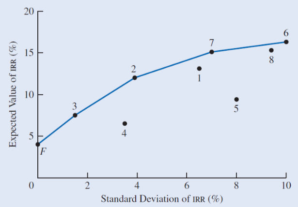
Risk vs. Return
Risk vs. return graph is a visual way to consider the risk (standard deviation) and the return (expected value).
- Risk (standard deviation \(\sigma\)) lies on the x-axis
- Return (expected value) lies on the y-axis
Note that the return is usually in the form on internal rate of return.
Example: risk vs. return graph
Notice that it’s less risky when SD is lower, but the return is less.
Also notice that the rate of return tapers off as SD increases meaning eventhough the return is larger, the risk is riskier.